Understanding Big O Notation: The Key to Efficient Algorithms

Understanding how to measure and optimize the performance of your algorithms is crucial. This is where Big O Notation comes into play. It's not just a theoretical concept but a practical tool that helps in assessing the efficiency of algorithms in terms of time and space complexity. Let's delve into this cornerstone concept of computer science.

What is Big O Notation?

Big O Notation is a mathematical representation used to describe the performance of an algorithm. Specifically, it measures the worst-case scenario of an algorithm's runtime or space requirements as a function of the input size. In simpler terms, it tells you how fast an algorithm grows relative to the input size.

Why is Big O Notation Important?

1. Performance Prediction: It helps in predicting how an algorithm will perform as the size of the input data increases.

2. Efficiency Comparison: It provides a way to compare the efficiency of different algorithms for the same task.

3. Bottleneck Identification: It assists in identifying potential bottlenecks in code, guiding developers in optimizing their algorithms.

Common Big O Notations

1. O(1) - Constant Time: Execution time remains constant regardless of input size.

2. O(n) - Linear Time: Execution time increases linearly with input size. Example: Linear search.

3. O(log n) - Logarithmic Time: Execution time increases logarithmically with input size. Example: Binary search.

4. O(n log n) - Linearithmic Time: Combines linear and logarithmic complexities. Common in efficient sorting algorithms like mergesort and heapsort.

5. O(n^2) - Quadratic Time: Execution time is proportional to the square of the input size. Common in algorithms with nested loops, such as bubble sort.

6. O(n^3) - Cubic Time: Execution time is proportional to the cube of the input size. Less common, but seen in certain algorithms involving three nested loops.

7. O(2^n) - Exponential Time: Execution time doubles with each additional input element. Seen in some recursive algorithms, especially those that solve the subsets of a set.

8. O(n!) - Factorial Time: Execution time grows factorially with the input size. Common in algorithms that compute all permutations of a set (e.g., the traveling salesman problem via brute-force search).

Image from the practicaldev.com

Understanding Big O Notation Through Practical Examples

To better grasp this concept, let's dive into this practical example, analyzing its Big O notation.

Analysis of the bubble_sort Function

Big O Analysis by Line:

1. Function Definition (Line 1): O(1) - Defining a function does not depend on the input size.

2. Length Calculation (Line 2): O(1) - Calculating the length of the array is a constant time operation.

3. Outer Loop (Line 3): O(n) - The outer loop runs n times where n is the length of the array.

4. Inner Loop (Line 4): O(n) - In the worst-case scenario (the array is in reverse order), this loop runs n-i-1 times per iteration of the outer loop. Over all iterations, this accumulates to nearly n times.

5. Comparison (Line 5): O(1) - Comparing two elements is a constant time operation. However, this line is executed once for each iteration of the inner loop.

6. Swap (Line 6): O(1) - Swapping two elements is also a constant time operation, executed for each iteration of the inner loop.

7. Return Statement (Line 7): O(1) - Returning the array is a constant time operation.

Overall Big O Calculation:

• The key to understanding the overall complexity lies in the nested loops (Lines 3 and 4). The outer loop runs n times, and for each iteration of the outer loop, the inner loop runs approximately n times in total (summing over all iterations of the outer loop).

• Therefore, the total number of basic operations (comparisons and swaps) is proportional to n * n, or n^2.

• While there are constant time operations within these loops, the overall time complexity is dominated by the most significant term, which in this case is n^2.

• As a result, the time complexity of the bubble sort algorithm is O(n^2).

More examples

1. O(1) - Constant Time: Accessing an Element in an Array

In Python, accessing an element in an array (or list) is a constant time operation. No matter how large the list is, accessing an element takes the same amount of time.

2. O(n) - Linear Search

When searching for an element in an unsorted list, you might have to look at every element once. This results in a linear time complexity.

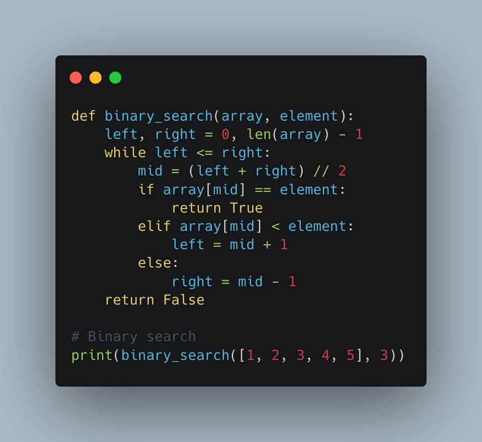
3. O(log n) - Binary Search

Binary search is a classic example of logarithmic time complexity. It splits the data in half with each iteration, significantly reducing the search time.

4. O(n log n) - Merge Sort

Merge sort is a classic example of an O(n log n) algorithm. It divides the array into halves, sorts each half, and then merges them back together.

5. O(n^2) - Bubble Sort

Bubble Sort is a simple sorting algorithm with quadratic time complexity. It repeatedly steps through the list, compares adjacent elements, and swaps them if they are in the wrong order.

6. O(n^3) - Cubic Time Example

A simple example of a cubic time complexity is a triple nested loop. Let's consider a case where we sum the product of triples of numbers from an array:

7. O(2^n) - Fibonacci Sequence (Recursive)

The recursive calculation of the Fibonacci sequence is a common example of O(2^n) complexity, where the function calls itself twice at each step.

8. O(n!) - Calculating Permutations

An O(n!) algorithm can be illustrated by generating all possible permutations of an array: